Time-Series Forecasting

Time-series forecasting takes a continuous period of time-series data as its input and forecasts how the data will trend in the next continuous period. The number of data points in the forecast results is not fixed, but can be specified by the user. TDgpt uses the FORECAST function to provide forecasting. The input for this function is the historical time-series data used as a basis for forecasting, and the output is forecast data. You can use the FORECAST function to invoke a forecasting algorithm on an anode to provide service. Forecasting is typically performed on a subtable or on the same time series across tables.

In this section, the table foo is used as an example to describe how to perform forecasting and anomaly detection in TDgpt. This table is described as follows:

Column	Type	Description
ts	TIMESTAMP	Primary timestamp
val	Integer	Measured value
past_co_val	Integer	Historical covariate
future_co_val	Integer	Future covariate

taos> SELECT * FROM foo LIMIT 2;
           ts            |   val | past_co_val | future_co_val |
================================================================
 2020-01-01 00:00:12.681 |    13 |           1 |             1 |
 2020-01-01 00:00:13.727 |    14 |           2 |             1 |

Syntax

FORECAST(column_expr, option_expr)

option_expr: {"
algo=expr1
[,wncheck=1|0]
[,conf=conf_val]
[,every=every_val]
[,rows=rows_val]
[,start=start_ts_val]
[,timeout=timeout_val]
[,expr2]
"}

1. column_expr: The time-series data column to forecast. Enter a column whose data type is numerical.
2. options: The parameters for forecasting. Enter parameters in key=value format, separating multiple parameters with a comma (,). It is not necessary to use quotation marks or escape characters. Only ASCII characters are supported. The supported parameters are described as follows:

Parameter Description

Parameter	Definition	Default
algo	Forecasting algorithm.	holtwinters
wncheck	White noise data check. Enter 1 to enable or 0 to disable.	1
conf	Forecast confidence level used for _FLOW and _FHIGH. End-to-end requests must use a value in (0, 1), such as 0.95.	0.95
every	Sampling period.	The sampling period of the input data
start	Starting timestamp for forecast data.	One sampling period after the final timestamp in the input data
rows	Number of forecast rows to return.	10
timeout	Maximum time to wait for the forecast request, supported since v3.3.6.5. The range is 1 to 1200 seconds.	60 seconds

• Three pseudocolumns are used in forecasting:
  • _FROWTS: the timestamp of the forecast data
  • _FLOW: the lower threshold of the confidence interval
  • _FHIGH: the upper threshold of the confidence interval. For algorithms that do not include a confidence interval, the _FLOW and _FHIGH pseudocolumns contain the forecast results.
• You can specify the START parameter to modify the starting time of forecast results. This does not affect the forecast values, only the time range.
• The EVERY parameter can be lesser than or equal to the sampling period of the input data. However, it cannot be greater than the sampling period of the input data.
• If you specify a confidence interval for an algorithm that does not use it, the upper and lower thresholds of the confidence interval regress to a single point.
• The maximum value of rows is 1024. Values above this limit return an error.
• Forecasting requires at least 10 input rows and supports at most 40,000. Some models have stricter limits.

Selecting CES, Theta, or ETS

Data characteristics	Recommended algorithm	Reason
The seasonal pattern is complex or does not fit a conventional additive or multiplicative pattern.	CES	CES can represent seasonal behavior with complex-valued states and can automatically select its model form.
The series has a clear long-term trend and relatively regular seasonality.	Theta	Theta is a compact trend-focused method; choose additive decomposition for stable seasonal amplitude and multiplicative decomposition for proportional seasonal amplitude.
You want an interpretable combination of error, trend, and seasonal components.	ETS	ETS can automatically select or explicitly configure additive and multiplicative components, with optional damped trend behavior.

Start with automatic selection (model=Z for CES or model=ZZZ for ETS) when the component structure is unknown. Theta multiplicative decomposition and any explicitly multiplicative ETS component require strictly positive input. For seasonal forecasts, set period and provide at least two complete periods of historical data.

Example

--- ARIMA forecast, return 10 rows of results (default), perform white noise data check, with 95% confidence interval 
SELECT _flow, _fhigh, _frowts, FORECAST(val, "algo=arima")
FROM foo;

--- ARIMA forecast, periodic input data, 10 samples per period, disable white noise data check, with 95% confidence interval
SELECT _flow, _fhigh, _frowts, FORECAST(val, "algo=arima,conf=0.95,period=10,wncheck=0")
FROM foo;

taos> select _flow, _fhigh, _frowts, forecast(i32) from foo;
        _flow         |        _fhigh        |       _frowts           | forecast(i32) |
========================================================================================
           10.5286684 |           41.8038254 | 2020-01-01 00:01:35.000 |            26 |
          -21.9861946 |           83.3938904 | 2020-01-01 00:01:36.000 |            30 |
          -78.5686035 |          144.6729126 | 2020-01-01 00:01:37.000 |            33 |
         -154.9797363 |          230.3057709 | 2020-01-01 00:01:38.000 |            37 |
         -253.9852905 |          337.6083984 | 2020-01-01 00:01:39.000 |            41 |
         -375.7857971 |          466.4594727 | 2020-01-01 00:01:40.000 |            45 |
         -514.8043823 |          622.4426270 | 2020-01-01 00:01:41.000 |            53 |
         -680.6343994 |          796.2861328 | 2020-01-01 00:01:42.000 |            57 |
         -868.4956665 |          992.8603516 | 2020-01-01 00:01:43.000 |            62 |
        -1076.1566162 |         1214.4498291 | 2020-01-01 00:01:44.000 |            69 |

Covariate Forecasting

TDgpt supports univariate forecasting and, since v3.3.6.6, historical covariate forecasting. Static covariates are not supported.

Only the moirai time-series foundation model is supported for covariate forecasting. If you want to perform covariate forecasting, you must set the algo parameter to moirai.

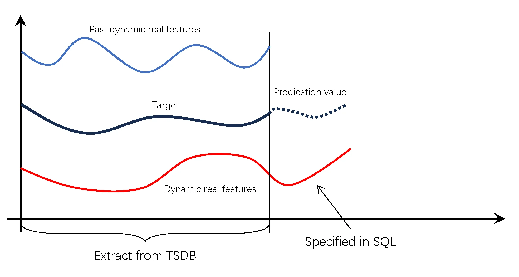
In the diagram above, there are two covariates and one target variable (also called the primary variable). Target is the forecasting objective, and Prediction value is the forecast result. Past dynamic real features represent historical covariates, while Dynamic real features represents future covariates.

Historical and future covariate data aligned with the same time window as the target variable are retrieved from the time-series database. Future covariate values corresponding to the prediction horizon must be provided directly in the SQL statement. Detailed usage is described below.

Historical Covariate Forecasting

Historical covariate forecasting is available in v3.3.6.6 and later.

When the forecast function takes a single column as input, it operates in default univariate forecasting mode. When multiple columns are provided, the first column is treated as the primary variable, and subsequent columns are treated as covariates.

All input columns must be numeric. Each forecasting query supports up to 10 historical covariate columns. The following SQL example demonstrates covariate forecasting:

SELECT _frowts, forecast(val, past_co_val, 'algo=moirai') FROM foo;

In this example, the first column (val) is the primary variable; subsequent columns (past_co_val) are historical covariates.

Future Covariate Forecasting

For future covariate forecasting, you must specify the future input values and their associated covariate columns.

Future covariate values must be provided directly in the SQL statement using array syntax within square brackets, with values separated by spaces.
The number of values must match the forecasting horizon; otherwise, an error will occur.

Future covariates use the prefix dynamic_real_. If multiple future covariates are used, they can be named sequentially as dynamic_real_1, dynamic_real_2, dynamic_real_3, and so on.

For each future covariate, the corresponding column must be specified:

• The column for dynamic_real_1 is defined via the parameter dynamic_real_1_col
• The column for dynamic_real_2 is defined via dynamic_real_2_col, and so on

In the example below, forecasting is performed on the val column. One historical covariate column past_co_val is provided, along with one future covariate column future_co_val. Future covariate values are supplied via dynamic_real_1, which contains 4 future values in the array. The parameter dynamic_real_1_col=future_co_val maps the future covariate to the future_co_val column.

select _frowts, forecast(val, past_co_val, future_co_val, "algo=moirai,rows=4, dynamic_real_1=[1 1 1 1], dynamic_real_1_col=future_co_val") from foo;

Built-In Forecasting Algorithms

• ARIMA
• HoltWinters
• Prophet
• Time-Series Foundation Model
• Complex exponential smoothing (CES)
• Theta
• ETS (Error, Trend, Seasonal)
• XGBoost
• LightGBM
• Multiple Seasonal-Trend decomposition using LOESS (MSTL)
• Long Short-Term Memory (LSTM)
• Multilayer Perceptron (MLP)
• DeepAR
• N-BEATS
• N-HiTS
• Patch Time Series Transformer (PatchTST)
• Temporal Fusion Transformer
• TimesNet